⌚ July 12, 2014
 Would you like to have a faster home network? Do you have any spare network interface cards (NICs) lying around unused? Do you run Linux?
If yes, then you can put your spare hardware to good use to increase the speed of your LAN and increase its fault tolerance. Link aggregation, also known as port trunking or bonding, lets you pair a group of network cards together so they operate as a single, faster logical network card.
Despite the intimidating name, link aggregation in Linux is inexpensive, simple to set up, and supported natively. No need for special vendor drivers or program recompilation. Once set up and running, operation is transparent to programs. Just use the network like you normally would.
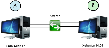
This article shows how to set up link aggregation in Linux Mint 17 and Xubuntu 14.04 using everyday, consumer-grade gigabit networking hardware. Stuff you might already have. Nothing fancy, complex, or exotic. Throughput boosts from 1 Gb/s to 2 Gb/s or 3 Gb/s depending upon the number of network cards and ports used.
Update December 20, 2016: With recent Linux distributions, such as Linux Mint 18.1, the “Making Changes Permanent” section using /etc/network/interfaces no longer works as described. Aggregation still works when set up manually or when using a script.
However, it will still work with a few changes as described in Link Aggregation in Linux Mint 18.1 and Xubuntu 16.04.
Overview
- Background and Theory
- What Link Aggregation Does
- What Link Aggregation Does NOT Do
- What Good Is Link Aggregation?
- What Do I Need? (The hardware)
- Setting Up the Hardware
- Setting Up Linux (Configuration)
- Making Changes Permanent
- Testing Speeds with netcat and FTP
- Monitoring with iftop
- How Fast? (Network arrangements and resulting throughput.)
- Testing Fault Tolerance
- Possible Bottlenecks
- Problems and Issues and How I Resolved Them
- What About Windows 7?
- Conclusion
The Background
Back in the days of dial-up modems that were limited to 3-5 KB/s, a variety of techniques were developed to increase the speed. One technique was often referred to as the “shotgun.” This implemented two modems, each operated in parallel at 5.6 KB/s, to produce an aggregated throughput of 11 KB/s. Both modems connected to an ISP and operated in parallel to almost double the speed.
Can the same idea be applied to today’s Gigabit Ethernet? For example, is it possible to add a second gigabit NIC to increase the throughput from 1 Gbps to 2 Gbps? How about a third NIC for 3 Gbps?
Yes, and Linux supports it natively. All it takes is extra network hardware and the time to edit some Linux configuration files.
Throughput, Links, and Transfer Rate. What’s the Difference?
I tend to use these terms loosely in this article, and sometimes I devise my own. For this project, I use throughput to describe the total MB/s available for use whether or not all is used. Compared to plumbing, think of throughput as how wide of a pipe through which water flows. More throughput in link aggregation means a wider pipe through which data travels.
I avoid the term bandwidth because this is technically a signaling metric expressed in MHz. For example, a category 6 network cable supports a bandwidth of 250 MHz, and category 6a cable supports a bandwidth of 500 MHz. These values express technical limits of the wires.
Transfer rate, expressed in MB/s, is how fast a single file transfers from one location to another. Real-world factors, such as hard drive speed and overhead, affect the actual transfer rate, which is different from throughput. Link aggregation might supply a throughput of 300 MB/s, but the transfer rate of a single file might be limited to 43 MB/s. Filezilla reports the final transfer rate after a file completes its transfer.
A link (my term) describes a single channel in an aggregated network. It consists of one network card connected to a switch using one cable. Two links, or two channels, use two network cards, each connected to a switch through two cables. Three links use three network cards and three cables.
Adhering to terms strictly can be counterproductive and confusing in some cases, so I try to present the concept at the risk of using some terms incorrectly. It is analogous to the terms number and numeral, which are two different things. A number is an idea, and a numeral is an expression of that idea. However, we tend to use the terms interchangeably.
The Theory
To help understand what we are trying to achieve with link aggregation, let’s examine a normal file transfer over a typical home network. Assume that this is the perfect network operating at full speed without any bottlenecks. We are using a gigabit network in its entirety: switches, cards, operating system support, and category 6 cable. Gigabit all the way.
A lone client connects to a server and downloads a file. Since the client has the server all to itself, the file downloads at the theoretical maximum of 1 Gbps. (About 100 MB/s assuming 10 bits transfer a single byte. This is typical for serial communications. Powers of 10 factor in some overhead and simplify conversions.)

Actual speeds might vary in real life, but this illustrates the point. During concurrent transfers, 1 Gbps throughput must be divided among all connected nodes. This causes the transfer rate per node to decrease.
In real life, other factors, such as overhead and hard drive speed, affect the transfer speed, but we are trying to understand the concept for now.
Sidenote: Bits or Bytes? Upper-case or Lower-case?
A lower-case b means bits, and an upper-case B means bytes.
b = bits
B = Bytes
This is very important since the two are often confused. To obtain a rough estimate of the theoretical maximum of how many bytes can be transferred over a 1 Gbps network, divide 1000 by 10 to get 100 million bytes (100 megabytes), per second. We express network speeds in powers of 10, not 2.
Gbps or Gb/s = Gigabits per second
Mbps or Mb/s = Megabits per second
MBps or MB/s = Megabytes per second
Since we are transferring files, it is usually easier to think in terms of bytes for file sizes, so the client downloads a file at the speed, or transfer rate, of 100 MB/s (100 megabytes per second). Real life affects this value greatly, but ignore real life for now.
With one client, the full 100 MB/s is available. But suppose a second client downloads files at the same time as the first client. Now, the throughput is shared between the two clients, giving each 50 MB/s. If four clients connect and download simultaneously, then the available throughput is split four ways, giving all four clients 25 MB/s. More clients means longer download times per client because the network speed is limited to 100 MB/s total, and it must be shared by all who connect.
What Link Aggregation Does
Is there a way to let multiple clients download at 100 MB/s (1 Gb/s) each simultaneously?
Yes, and this is the purpose of link aggregation. Where one NIC allows a maximum of 1 Gbps that must be split into 500 Mb/s per client for two clients, two NICs bonded together will provide a maximum of 2 Gbps (200 MB/s) so each client will download at 1 Gbps (100 MB/s) simultaneously. This is because the available throughput provided by the server has doubled by using two network cards.

Doubling the throughput doubles the possible transfer rates per client up to the 1 Gpbs limit, but only for concurrent file transfers.
Adding a third card will triple the aggregate throughput.

To take full advantage of triple links and ~300 MB/s throughput, multiple files must be transferred simultaneously. This makes link aggregation an excellent choice for media servers connected to many clients.

Wireless devices, netbooks, game consoles, and media clients who all possess only one network port can make good use of this configuration. The server uses three links in order to supply enough throughput to feed all connected devices without any noticeable slowdown on the client side.
Four will quadruple, and so on. However, there comes a point when other computer hardware, such as hard drive speed, will bottleneck the transfer rate more than the network connection itself.
What Link Aggregation Does NOT Do
First, let’s clear up a common misunderstanding regarding link aggregation:
“If one NIC lets me transfer a file at 100 MB/s, will two NICs transfer the same file at 200 MB/s? Will the transfer rate double for a single file transfer?”
No, not really, but if it does, consider it an unexpected bonus. Individual file transfers are still limited to about 1 Gbps (100 MB/s) per transfer. Link aggregation only allows more 1 Gbps transfers to occur simultaneously before splitting up the available throughput among connected clients. Think of it in terms of channels or lanes. Link aggregation only increases the number of lanes, not the speed per lane.

Comparison with a vehicle traffic lane helps understand the concept of interface bonding. Adding more lanes does not increase the speed limit. It only allows more of the same speed to travel simultaneously.
As an analogy, think of a vehicle highway with a speed limit of 80 (use whatever units you prefer). Cars traveling in one direction (one lane) must line up and travel in a single row (for one direction). And no, these cars cannot pass the slowpokes who talk on cell phones and weave across the line.
If we add a second lane to the highway (same direction). More cars can travel simultaneously on two parallel lanes, but the speed is still limited to 80 per lane.
Link aggregation operates the same way. Two or three network cards might double or triple the available lanes, but each network lane (network port) is still limited to 1 Gbps. Instead of a single file transfer occurring through a single network port, it is distributed across all ports (lanes). However, the single file transfer speed rarely exceeds 1 Gbps despite distributed load balancing across multiple network cards. When transferring a single file using a three-card bond, the file will usually be limited to about 1 Gbps maximum despite the actual frames being sent across all three network cards. The three cards provide a total of 3 Gbps maximum throughput, but the leftover 2 Gbps will remain unused during the single file transfer.
Of course, there are exceptions. For example, synthetic benchmarks and some file transfers will exceed the 100 MB/s limit due to the distribution across network cards.
With three NICs bonded, I have seen file transfers reach 140-208 MB/s for a single file, but this was only possible as long as the entire network path was tripled between two computers: three NICs in each computer, six switch ports, and three physical cables per computer. It tended to be the exception, not the norm.
Synthetic benchmarks using netcat will top out the measured transfer rate, but these are synthetic numbers, not real-life numbers. With a triple-network path transferring multiple netcat tests, I have measured a maximum speed of 336-344 MB/s, but this is a synthetic benchmark designed to measure available throughput, not real life file transfer rates.
Another example involves Filezilla connected to the Filezilla server or vsftpd. Filezilla lets you download multiple files simultaneously via FTP, and the transfer rates of each transfer are displayed. If downloading three files at once, the available throughput is divided among the three files. With the standard gigabit network, each file transfers at about 33 MB/s, but with triple-link aggregation, Filezilla transfers all three files simultaneously at the full 100 MB/s each — taking into account other real-world factors.
What Good is Link Aggregation?
“Okay, I am a single user connecting two computers together to transfer files between them one at a time. If link aggregation does not offer any real speed boost doing that, then what good is it?”
Multiple Connections With Little Speed Loss
Single file transfers or one-at-a-time transfers do not benefit much from link aggregation, but multiple connections and file transfers do. Some transfer rate increase might be apparent, but link aggregation shines in the area of multiple simultaneous transfers where several clients connect and download concurrently. Having more network lanes available allows all clients to enjoy faster download speeds.
Examples include a personal media server or network attached storage where multiple devices or users connect.
Redundancy
Another advantage is redundancy. The physical links (cables) can be spread across multiple switches. If one switch fails or a cable is torn or disconnected, the transfer continues but at slower speeds until the issue is resolved.
Of course, redundancy might not be needed if all computers are located close together, such as on the same desk or in neighboring rooms. Due to their close proximity, whatever happens to one cable or switch might happen to the other also. It depends.
Load Balancing
This balances the network load across multiple network cards for more even performance and better throughput. Rather than making one card do most of the work, let the other cards share the fun by distributing the workload among them.
It’s Inexpensive and Well-Supported in Linux
With Linux, link aggregation is simple and low-cost. You can use existing consumer-grade networking hardware. While more expensive 802.3ad LACP (Link Aggregation Control Protocol) hardware is available, it is not necessary, making this perfect for personal use.
What Do I Need?
“Whew, that was a lengthy explanation! So, what hardware do we actually need to create a link aggregated network? “
Link aggregation is an even lengthier topic that accommodates a variety of networking scenarios, but we want something simple, fast, reliable, and compatible with other devices, so this article builds a simple link aggregated network using the default round-robin algorithm.
It boils down to switches, cables, network cards, and editing a few configuration files in Linux. With Linux, you should be able to use any hardware you have. Here is what I used with resounding success:
- TRENDnet 8-port Gigabit Switch TEG-S80g (Two for fault tolerance experiments)
- Syba Dual-port Gigabit NIC (Two ports on one PCIe x1 card to save space)
- Cat 6 colored cables (For easier cable management)
- Other generic gigabit NICs and cables gathering dust
Keep in mind that you do not need to use the same hardware that I used in order to make link aggregation work. This is what I used, and it worked well for me. Of course, if your hardware is inadequate, then you might need to invest in new hardware.
TRENDnet 8-port Gigabit Switch (x2)
I needed a switch with more ports, so I chose this brilliant performer:

The original plan was to split the network path into two lanes, which is why I used two switches. These are extremely energy-efficient switches (3.5W max each), making them ideal for home use. They are small, run cool, and made of metal. The LEDs are located on the front panel while the power and network ports are located on the back. Very convenient. Simply plug them in and go. No configuration necessary. 16Gb/s total full duplex per switch.

Back view showing eight gigabit ports and the power connector.

The TRENDnet switches can be chained together to act as a single switch. This leaves 14 available ports. If doing this, use one cable to link them or else the network will not work.
Syba Dual-port Gigabit NIC
Many new motherboards no longer have PCI slots, so I needed a PCIe NIC. Why not use a dual-port NIC?

Linux detects and uses this card with 100% compatibility. No driver installation needed. A Linux plug-and-play dream come true! Both gigabit ports operate at full duplex. Combined with the existing network port on the motherboard, the test computer this was installed in supplied a 3Gbps throughput. The cost of this card was identical to two separate single-port cards.

Generic, inexpensive gigabit single-port NIC. Had to find a motherboard with a PCI slot in order to use it. 100% Linux compatible.
Here are additional hardware details:
Network Cards
You need physical network cards.
Throughput will not increase magically from 1Gbps to 2Gbps or 3Gbps using a single network port. You will need more hardware.
If your motherboard already has a network port, you can use it with an additional network card for two ports. Some network cards contain multiple ports. I used dual-port cards (shown above) with excellent results. A dual-port card combined with the motherboard port provides three network ports per computer for a total of 3 Gbps available throughput. Again, this does not mean that files will transfer at 3 Gbps per file, but three files will transfer at about 1Gbps each simultaneously.
These ports will be bonded together into a single logical network interface within Linux, so data will flow through all three ports in parallel.
Switches
Use unmanaged 1 Gbps, full-duplex switches. Do not use routers. Even though link aggregation is possible with routers, switches are better suited for this task.
802.3ad Is Not Necessary
The networking world has its own aggregation standard clearly defined as the Link Aggregation Control Protocol (LACP). Professional-grade networking routers and switches supporting 802.3ad offer additional port trunking features, but they are prohibitively expensive and overkill for this project.
Those features are not needed. You can perform full-duplex link aggregation using inexpensive switches with Linux. Hardware does not need to support LACP. This project is for personal use, and the result will probably be more than enough for the typical private LAN.
I used two TRENDnet unmanaged gigabit switches. These are fantastic switches because they are made of steel, they run cool to the touch, they consume less than 3.5W of power each, and each has a maximum throughput of 16 Gbps (2 Gbps full duplex per port x 8 ports = 16 Gbps).
Full Throughput
To reap full benefits, you will want the path between nodes (computers connected to your network) to contain the same “width” or number of lanes throughout. For a dual-lane setup, you will need two network ports per computer, and two cables connected to each computer. If using a triple setup, each computer will need three network ports and three cables each. A single switch will work.
Most important is to use Gigabit Ethernet throughout. Gigabit switches. Gigabit network cards. Category 6 cables. Chances are that you already have a few gigabit NICs gathering dust, so this should not be a problem. Avoid mixing with Fast Ethernet (100 Mbps) or slower. Otherwise, what’s the point? In theory, slower network cards should bond with Gigabit Ethernet, but I have not tried this. For best results, stick to one standard for the entire LAN.
It is perfectly fine to connect slower devices, such as game consoles, wireless access points, toasters, and vacuum cleaners, to the bonded network. They will communicate at their slower speeds.
Why Two?
Link aggregation will function with a single switch, but you will need at least two switches for true fault tolerance. Cables from one lane connect to one switch while the other lane connects through the second switch. If one switch fails (never has) or one cable disconnects (never did), the other switch continues functioning.
Will Link Aggregation Work With One Switch?
Yes. You do not need two or three switches. If the switch is full-duplex and full throughput, such as the TRENDnet above as an example, you can connect all network cards to the same switch and enjoy the maximum throughput. Use at least an 8-port switch because those ports will be used up quickly.
In fact, I prefer the single switch approach for best compatibility. Dividing the lanes among separate switches introduces problems with single-port nodes (discussed later). These issues do not occur with a single switch.
If you want to experiment with fault tolerance using two switches and then settle on a single-switch design, use two switches. They can be connected together to act as a single switch using one network cable between them. Do not use two network cables to connect the switches or else the network will not work.
I did this thinking that two cables would double the throughput between switches, but no success. The activity lights flash incessantly, and no networking is possible. Use one cable to connect the switches.
Colored Cables
With so many connections, you can expect cable clutter! So, to help manage the cable mess that is bound to happen, use colored cables, and let each color represent one computer. This makes it easier to trace a pair of cables to its computer.
Use category 6. Cat 5e should work, but cat 6 is built to higher standards.

Even dull-colored cables are better than no color at all. You will thank yourself many times later.

One color per computer. Blue cables were connected to all network ports on this test computer.
Setting Up the Hardware
For simplicity, start with two computers and one switch. Once the two computers communicate with each other, we can easily expand the system.
Install all network cards in two computers. Color code each computer by cable color.
Checking the NICs In Linux
Linux Mint 17 and Xubuntu 14.04 were the two test machines. To see what Linux sees, boot into Linux and run ifconfig.
ifconfig
All network interfaces should appear whether or not they are configured. Linux must detect and display a NIC here before you can use it. If an installed NIC does not appear in the ifconfig listing, then you cannot bond it with other network interfaces. Turn off the computer and try moving the NIC to another slot on the motherboard.
This happened to me. For reasons unknown, one NIC would not work in two PCIe x1 slots that I tried. BIOS and Linux refused to detect it. But when the NIC was moved to a PCIe x16 slot, it worked. Strange…
Also, ensure that all network cards operate as they should individually at this point. We do not want to bond a 1 Gbps interface and malfunctioning 100 Mbps interface together and then wonder why the transfer rate is slow. Ping each computer from each computer using individual connections. You will need to set up separate network connections for this using Network Settings in Linux Mint 17, but these can be deleted once finished.
Install ifenslave
ifenslave is the program that bonds network interfaces together. We need it, so let’s install it now on every computer.
sudo apt-get install ifenslave
Temporary Bonding
Before we make the bonding boot-time permanent, let’s see if it will work per session. This means creating the bond using the terminal. Rebooting will clear any interface bonds.
First, decide on a network ID. For this example, we will use 192.168.2.0. The “2” network to avoid confusion with the well-known 192.168.1.0.
On each computer, identify the individual network interfaces using ifconfig. This will be something like eth1, eth2, and so on. It’s okay if the numbering varies between computers, but ensure that the interfaces you want to bond together are detected.
Here is a brief overview of commands for the bonding process:
sudo modprobe bonding
sudo ip addr add 192.168.2.10/24 brd + dev bond0
sudo ip link set dev bond0 up
sudo ifenslave bond0 eth0 eth1
View bonding info once complete:
cat /proc/net/bonding/bond0
Install the bonding Linux Module: sudo modprobe bonding
Linux needs the bonding module, so install it from the terminal using modprobe.
sudo modprobe bonding
It is possible to append a range of options, such as the mode and delays, but keep things simple for now. By default, bonding uses the round-robin load-balancing mode (mode 0), which is plenty fast and well-suited for our simple needs.
Set Up the Interface
sudo ip addr add 192.168.2.10/24 brd + dev bond0
The bonded interface will be recognized by the name bond0, and it will be given a static IPv4 address of 192.168.2.10 as specified in the command line. You are free to change these to whatever values you might need for your network.
bond0 is the name of the logical address that we will later enslave the physical network interfaces to. Once bond0 is up and running, we can identify and monitor it as bond0.
NOTE: It is not necessary to set up IP addresses for the individual physical interfaces (eth1, eth2, and so on) even though you can. Bonding will function whether or not the individual interfaces have IP addresses. I never bothered assigning IP addresses for the NICs aside from testing. What matters is the IP address of bond0.
Enable the bond0 interface
sudo ip link set dev bond0
Create the Bond
sudo ifenslave bond0 eth0 eth1
This bonds physical interfaces eth0 and eth1 to the logical bond0.
Three NICs
sudo ifenslave bond0 eth0 eth1 eth2
Four NICs, different names
sudo ifenslave bond0 eth1 eth2 eth3 eth5
Viewing Bonding Information
If all went well, you should be able to view the status of the bond.
cat /proc/net/bonding/bond0
Replace bond0 with the name of whatever logical bond you created. You should see something like this for a bond of three network interfaces:
Ethernet Channel Bonding Driver: v3.7.1 (April 27, 2011)
Bonding Mode: load balancing (round-robin)
 MII Status: up
 MII Polling Interval (ms): 0
 Up Delay (ms): 0
 Down Delay (ms): 0
Slave Interface: eth0
 MII Status: up
 Speed: 1000 Mbps
 Duplex: full
 Link Failure Count: 0
 Permanent HW addr: 23:fe:93:2c:67:55
 Slave queue ID: 0
Slave Interface: eth1
 MII Status: up
 Speed: 1000 Mbps
 Duplex: full
 Link Failure Count: 0
 Permanent HW addr: 6e:8a:ce:25:23:22
 Slave queue ID: 0
Slave Interface: eth2
 MII Status: up
 Speed: 1000 Mbps
 Duplex: full
 Link Failure Count: 0
 Permanent HW addr: 08:0a:cd:35:63:26
 Slave queue ID: 0
Important Lines:
Bonding mode - What mode the bond is operating in. There are seven modes, 0-6.
MII Status - Whether the interface is up or down. If down, it will not be used.
Speed - Ensure 1000 Mbps (1 Gbps) per interface
Duplex - You want full duplex for maximum speed
Run ifconfig to see more details.
bond0     Link encap:Ethernet  HWaddr 23:fe:93:2c:67:55
 inet addr:192.168.2.10  Bcast:192.168.2.255  Mask:255.255.255.0
 inet6 addr: fe80::96de:80ff:fe2b:4544/64 Scope:Link
 UP BROADCAST RUNNING MASTER MULTICAST  MTU:1500  Metric:1
 RX packets:5499 errors:0 dropped:0 overruns:0 frame:0
 TX packets:2754 errors:0 dropped:0 overruns:0 carrier:0
 collisions:0 txqueuelen:0
 RX bytes:917369 (917.3 KB)  TX bytes:459603 (459.6 KB)
eth0      Link encap:Ethernet  HWaddr 23:fe:93:2c:67:55
 UP BROADCAST RUNNING SLAVE MULTICAST  MTU:1500  Metric:1
 RX packets:2166 errors:0 dropped:0 overruns:0 frame:0
 TX packets:586 errors:0 dropped:0 overruns:0 carrier:0
 collisions:0 txqueuelen:1000
 RX bytes:420088 (420.0 KB)  TX bytes:39103 (39.1 KB)
eth1      Link encap:Ethernet  HWaddr 23:fe:93:2c:67:55
 UP BROADCAST RUNNING SLAVE MULTICAST  MTU:1500  Metric:1
 RX packets:1667 errors:0 dropped:0 overruns:0 frame:0
 TX packets:1085 errors:0 dropped:0 overruns:0 carrier:0
 collisions:0 txqueuelen:1000
 RX bytes:248742 (248.7 KB)  TX bytes:210449 (210.4 KB)
eth2      Link encap:Ethernet  HWaddr 23:fe:93:2c:67:55
 UP BROADCAST RUNNING SLAVE MULTICAST  MTU:1500  Metric:1
 RX packets:1666 errors:0 dropped:0 overruns:0 frame:0
 TX packets:1083 errors:0 dropped:0 overruns:0 carrier:0
 collisions:0 txqueuelen:1000
 RX bytes:248539 (248.5 KB)  TX bytes:210051 (210.0 KB)
The interesting point here is that all network interfaces will share the same MAC address. eth0, eth1, and eth2 are listed as slaves (SLAVE) while bond0 is listed as the master (MASTER). bond0 is the only interface with a static IP address, which is the IP address for this test computer.
Set Up Other Computers
Now, perform the same setup for the other computer. It is fine to use the same bond0 name, but use a different IP address. Single-port computers do not require bonding. They will communicate with a link aggregated network as-is.
Ping Testing
With both computers configured and connected to the same switch, see if they can ping each other. From each computer, ping the bond0 IP address of the other.
Bonding Modes
The default round-robin mode 0 works best for me, but your results might vary. Try them out. Keep in mind that changing modes requires changing them for all computers to truly see what is possible. You will need to bring the network interfaces down, edit, and then bring the network interfaces back up. Or you can simply reboot. Different modes are designed to handle various situations, so transfer rates might actually decrease for some modes. Here is a brief listing:
Mode
0   Round Robin (Default. Used in this article. Works well.)
1   Active Backup
2   XOR Balance
3   Broadcast
4   802.3ad. Requires an 802.3ad switch.
5   Transmit Load Balancing
6   Adaptive Load Balancing
For more information about bonding modes, have a look at the LiNUX Horizon Bonding page.
Making the Changes Permanent
The settings so far will not persist between reboots, so to make the changes automatic, edit two files:
-
/etc/modules
-
/etc/network/interfaces
/etc/modules
This loads the bonding module at boot time. Open /etc/modules and append bonding on a line of its own. That’s it. Save and close. Do this for all computers using link aggregation.
sudo gedit /etc/modules
# /etc/modules: kernel modules to load at boot time.
#
# This file contains the names of kernel modules that should be loaded
# at boot time, one per line. Lines beginning with "#" are ignored.
# Parameters can be specified after the module name.

lp
rtc
bonding
Options can be added on the same line as bonding:
bonding mode=5
By default, with no options specified, bonding uses the round robin algorithm (mode 0). Specifying mode=5 would cause the bond to operate using transmit load balancing. Consult online resources for details because this can become a highly-specialized topic that exceeds the scope of this project. For my uses, round robin is perfect, so no modification is necessary.
/etc/network/interfaces
This sets up the bond0 network interface at boot time. ifenslave must be installed. Open and edit this file with a text editor.
sudo gedit /etc/network/interfaces
auto bond0
iface bond0 inet static
address 192.168.2.10
netmask 255.255.255.0
network 192.168.2.0
gateway 0.0.0.0
up /sbin/ifenslave bond0 eth1 eth2 eth3
down /sbin/ifenslave -d bond0 eth1 eth2 eth3
Edit this for each computer using link aggregation. Specify the network interfaces as they are named per computer. Each computer must have a unique IP address. The settings given here are examples, so change them to meet your needs.
Save and close. Reboot, and bond0 should be automatic. Use ifconfig to check. If the boot time is slow and seems to stall, then there is probably an incorrect line in /etc/network/interfaces and you will need to correct it by booting into root mode. A slow boot usually occurs because one or more of the specified interfaces for ifenslave cannot be found for whatever reason. Boot to root, use ifconfig to double-check the interface names, and edit /etc/network/interfaces with the correct values.
Red Hat users will need to use a slightly different interface configuration. The method shown here applies to Debian-based distributions.
Testing Speeds With netcat
Netcat tests the raw throughput possible. What is the maximum throughput possible using link aggregation? Netcat will fill the pipes with bits, and you can use iftop to measure the throughput.
Other tools, such as iperf, will also work, but I chose to use one tool for consistency and time instead of a wide range of tools. I settled on netcat for no particular reason other than all netcat tests do nothing more than send a stream of zeroes from one computer to /dev/null on the second computer. To the best of my knowledge, no compression is in effect, so even though zeroes are being sent and received, they are recorded in their entirety.
Please note that netcat results do not reflect real world transfer times, so even though iftop and netcat might report a total throughput of 336 MB/s using three lanes, that does not mean you will transfer files at 336 MB/s. Other factors affect the transfer rate. Hard drive speed, processing power, and protocols, for example, will limit the real world transfer rates.
netcat Setup
Netcat requires a terminal running in each computer, and each runs a different command. One computer listens for traffic on a specific port, and the other computer sends traffic over the network using that port.
On computer B, the listening computer, run this command:
nc -l 11111 > /dev/null
nc
Surprise! The netcat program is called nc in Linux.
-l 11111
Listen for traffic on port 11111. You may chose any unused port that you find convenient. Keep in mind that the sending computer must transmit on the same port entered here.
> /dev/null
Redirect all incoming data to the great blackhole of Linux. Translation: Discard all received bits. This method bypasses any storage medium, so hard drive limitations have no effect. We want to eliminate as many bottlenecks as possible in order to test the raw throughput.
Go ahead and press Enter to run the command. Computer B will enter listening mode and wait for incoming data.
On computer A, the sending computer, we enter the command that transmits zero data to computer B. We will use the trusty dd command to generate the data stream and pipe it to netcat to send the data stream to the proper destination.
dd if=/dev/zero ***=1073741824 count=4 | nc -v 192.168.2.10 11111
dd if=/dev/zero ***=1073741824 count=4
This generates exactly 4,294,267,296 zero bytes, or 4 GB. 2 ^ 32. A power of 2. Change the count to another value to adjust the number of gigabytes used. 8 and 16 are good values. I used gigabytes because link aggregation causes fast data transmissions, and anything smaller will be over before you know it. I want enough data to travel over the network over a given amount of time so it will stabilize enough for iftop to report a consistent measurement. Small bursts of 1 GB or 100 MB are useless because they complete too fast to gauge.
nc -v 192.168.2.10 11111
The generated data must be sent to the listening computer, so we pipe it to netcat. The IP address must be the IP address of the bond0 interface on the destination computer. 192.168.2.10 is an example. The port 11111 is the same port we specified in nc -l 11111 > /dev/null. The ports must match!
Maxing Out the Network. One netcat connection will rarely use the full throughput possible with link aggregation. Like a file transfer, a single netcat connection will usually be limited to 116 MB/s or a little faster, such as 120-140 MB/s.
We want to test the limits of bond0, so we need to create multiple netcat connections and run them simultaneously either manually or with scripts. It will take two or three netcat instances to see iftop report 280-336 MB/s with three network lanes.
To accomplish this, simply listen on different ports and send to those ports.
On the listening computer, run each command in a separate terminal:
nc -l 11111 > /dev/null
nc -l 11112 > /dev/null
nc -l 11113 > /dev/null
On the sending computer, run each command in a separate terminal:
dd if=/dev/zero ***=1073741824 count=4 | nc -v 192.168.2.10 11111
dd if=/dev/zero ***=1073741824 count=4 | nc -v 192.168.2.10 11112
dd if=/dev/zero ***=1073741824 count=4 | nc -v 192.168.2.10 11113
The IP address is the same in each command because we are sending data to the same listening computer, but the ports must be unique in order to monitor data for each port separately.
Each individual netcat transfer will occur at a much lower transfer rate, say 43-90 MB/s depending upon how many netcats are running, but when summed, the total should be close to what iftop reports with bond0. For two netcat transfers across three lanes, iftop will report ~280 MB/s, but each netcat will report a transfer rate of ~140 MB/s each. Running one netcat will report a transfer rate of ~113-126 MB/s.
“What About the Linux Mint System Monitor? Why are the values different there?”
No matter how many network monitors you run simultaneously, they will all report different values. Perhaps they are not updating the same value at exactly the same moment in time? Regardless, the reported values should be within a close range of each other. iftop might report 93 MB/s in real time while slurm reports 110 MB/s in real time while System Monitor reports 84 MB/s in real time while netcat reports the final transfer rate of 101 MB/s after the transfer completes. Netcat tends to produce the most accurate and consistent results closest to real life transfer, which is why I chose to use it for the tests.
Testing Real Speeds With FTP
Netcat is a synthetic benchmark. How fast are real file transfers? If I copy a file from one computer to another using link aggregation, how fast will it be?
FTP is a good choice because the FTP protocol is and simple and fast with little overhead. Other protocols, such as SSH, are slower and introduce extra overhead. To measure the fastest file transfer rate, I set up vsftpd and measured rates and times using Filezilla on computers with quad-core processors and SSD drives to reduce bottlenecks.
Monitoring With iftop
You can monitor any network interface in the bond using iftop. eth0, eth1, eth2, or whatever interface. It does not matter. However, iftop will only report the transfer rate for the monitored interface.
If eth0 is a slave in the bond and you monitor it with iftop, only the rate of eth0 is measured. This means that the traffic flowing through the other slave interfaces will be ignored.
To monitor the total throughput, we need to monitor the logical interface, bond0, itself. This reports the total, aggregate throughput of all interfaces used in link aggregation.
sudo iftop -Bi bond0
The -B option displays in Bytes per second, not bits per second. The following numbers are measured in MB/s using this command.

iftop running on the sending computer. It is monitoring all network traffic flowing through the bond0 logical interface. Here, the sending computer performing netcat tests by sending data to two different computers simultaeously.
Only one iftop is allowed per terminal window, so to monitor multiple interfaces, open multiple terminals and run a different instance of iftop in each one that monitors a different interface. One iftop monitors bond0, a second monitors eth1, and a third monitors eth2, for example.
sudo iftop -Bi eth1   <-- Run in its own terminal
sudo iftop -Bi eth2   <-- Run in its own terminal
How Fast?
So, what kind of throughput is possible? Here is a list of network configurations along with tested speeds. I used two types of tests: Netcat and FTP. FTP tests were fairly consistent over time because they are more hard drive dependent. If a 5400 RPM laptop hard drive only supports a 26 MB/s write mode, then the maximum transfer rate for a file to that drive is limited to 26 MB/s no matter how much network throughput is available.
Filezilla usually hovers around a 60-97 MB/s transfer rate for SSD hard drives whether using two or three network lanes. It was so consistent that I eventually quit measuring FTP transfer rates. Netcat transfers were a different matter, so I focused on them.
113 MB/s

Basic configuration like any other LAN. The baseline. Netcat maxes out at 113-116 MB/s.
144-175 MB/s

Adding a second network lane does not always double the throughput as you might expect, but it usually does.
With two lanes, the throughput tops out at 175 MB/s. In some instances, 206 MB/s was measured, but 175 MB/s was more consistent. Strangely, a few single FTP file transfers actually reached 144 MB/s.
With rsync, there was absolutely no speedup in transfer rates. An rsync backup was no faster with link aggregation than without. Same time. Same speeds. Yes, SSH was used with rsync.
116 MB/s

Testing two TRENDnet switches to see if they could be chained in series.
Would there be any loss of speed? None at all. The TRENDnet switches can be connected in series and still transfer files at the full 90-116 MB/s. After all, there is only one network lane through which data flows. With two 8-port switches, this effectively creates a single 14-port switch.
116 MB/s

The power of three! …maybe not.
Each computer contains three NICs and three cat 6 cables connected to separate switches. The switches are connected together in a series using one network cable.
The result? 116 MB/s transfer rates that are no faster than using one network lane. It’s the choke point. Data must travel between the switches, and it is limited to a 1 Gbps connection. This nullifies any benefits gained from link aggregation.
Logic would ask, “Why not connect an extra cable between the switches for 2 Gbps?”
But this does not work. In fact, the network becomes unusable.

This doesn’t work the way you think it would.
Each switch’s activity LED flickers constantly per connection in the absence of data transfers. Computers cannot ping each other. This effectively kills the network. Returning to a single cable returns the network to normal.
223 MB/s
2 : 3
Throughput is limited to the slowest link. In this case, A connects using two lanes. This limits the throughput to 2 Gbps for A even though B can operate at the full 3 Gbps.
Strangely, this configuration often reached 223 MB/s. 175 MB/s is usually typical for two lanes.
Transferred four 8 GB file simultaneously from SSD to SSD with a sustained throughput of 223 MB/s.
Transferring a 16 GB file using SSH was the same as always: 87 MB/s.
296 MB/s

Truly fast! But no switch fault tolerance.
This simple 3:3 arrangement produces some of the fastest results. With three network lanes, we begin to see impressive throughput numbers that exceed the capabilities of most computer hardware. Yes, link aggregation will work with a single switch. This yields a total of 3 Gbps potential throughput from A to B and back. The entire path from A to B must be “three.”
Link aggregation scales well. Adding a second lane doubles the throughput and three lanes triple the throughput. Almost. Due to overhead, the actual maximum throughput will be less. 290 MB/s is in the correct range of 275-303MB/s for three lanes.
If the switch goes down, no network. But if one or two cables are disconnected, file transfers will continue uninterrupted but only as fast as the remaining connections allow.

System Monitor running in Linux Mint 17 on the sending computer (A) during multiple netcat transfers from A to B. It reports 296.2 MB/s just like iftop.

System Monitor tended to hover just under 300 MB/s. I was expecting a 280 MB/s transfer rate with three links, so the 299 MB/s result is a welcome bonus.
314 MB/s

Speedy fault tolerance!
The two switches operate in parallel. If one fails, network activity continues uninterrupted but with less throughput. Restoring the failed switch increases the throughput to its max again.

In some cases, 321 MB/s was reached. This snapshot was taken shortly after the transfer started, but it tended to hover around this value for its duration.

System Monitor also reports 322 MB/s. One transfer was already in progress. When the second transfer was started, the graph jumped to report the higher value.
300+ MB/s speeds were typical. Remember, this does not mean that individual files transferred at 300 MB/s. They tended to transfer around 90-120 MB/s. However, this arrangement allows multiple, simultaneous file transfers of 90-120 MB/s each.
Two netcat transfers will operate at 153-155 MB/s each, but no single netcat operated at 300 MB/s.
Here, two netcat transfers are achieving 172 MB/s and 162 MB/s for a total of ~333 MB/s. These number mostly occur during synthetic benchmarks such as this. Real file transfers are more variable and tend to be limited by other computer hardware factors, such as slow hard drives.

~253 MB/s is more typical. Especially during actual file transfers.
This arrangement has a serious flaw: Single-port devices cannot use the network. They will rarely ping, and file transfers either timeout or are limited to 40 KB/s. The solution is to connect the two switches together with another network cable, but this drops the maximum throughput to 280 MB/s.
FTP. What kind of speeds are possible. Are three lanes truly faster? I compared the time it took to transfer the same three files of typical sizes over one lane and then over three lanes. Filezilla reported the final speeds and time.
One Lane, 3 Simultaneous FTP Transfers
         Size  Time

File 1:  247M  6s
File 2:  245M  6s
File 3:  338M  7s

Time to complete: 7s
Three Lanes, 3 Simultaneous FTP Transfers
File 1:  247M  3s
File 2:  245M  3s
File 3:  338M  4s

Time to complete: 4s
The files transferred in parallel, which is why we measure the longest times. 4s versus 7s. A 3-second difference. While link aggregation does not produce instantaneous file transfers (unless the files are small), the time saved becomes more apparent with larger files.
FTP With Multiple Drives
I tested simultaneous FTP transfers with files from multiple drives: SSD and two 7200 RPM. All three files were transferred to a Samsung EVO SSD located on the destination computer.
File 1:  96 MB/s
File 2:  70 MB/s
File 3:  70 MB/s

Sustained throughput: 236-244 MB/s
These numbers are reasonable. File 1 originated from an SSD, and its single file transfer rate is 96 MB/s. this is about the limit for single transfers. Again, link aggregation does not increase the transfer rates of individual files (not much, at least), but it allows more of them.
The two 70 MB/s transfers were slower because that is the read limit of the two 7200 RPM drives used. Link aggregation will not speed up your hard drives. These three files transferred as fast as they could without a drop in throughput. Had this been a single 1 Gbps connection, the files would have averaged about 33 MB/s each, and the total transfer time would have increased.
Yes. This is fast!
175 MB/s

Can you spot the error?
Two switches. Three NICs per computer. But the throughput is limited to 175 MB/s. Why?
Connections matter! Each switch is throttled by a 1 Gbps choke point. Two of these offer a total throughput of 2 Gbps, effectively the same as a dual-lane network. The lowest common denominator determines the maximum throughput available.
The correct method is to connect two lanes with one switch and the third lane to its own switch.

Now, we see 314 MB/s throughput again.
280 MB/s – Best Compromise
Highest compatibility with devices containing any number of network ports. Still fast at 280 MB/s.
This is the arrangement that works best for me. With the two switches connected to each via a single network cable, single-port and dual-port devices can use the network.
In this scheme, we see a third, dual-lane test computer connected. A and B have a throughput between themselves of 280-290 MB/s, but the dual-lane computer has a throughput of 175-180 MB/s.

iftop running on the sending computer (A) monitoring bond0. In this case, the total transfer rate of two simultaneous netcat transfer tests to two different computers reached 338 MB/s with this configuration. The 200 MB/s rate was achieved through two computers linked by three lanes, and the 137 MB/s transfer occurred from A to a dual-lane computer as shown in the picture above.

System Monitor in Linux Mint 17 on the sending computer (A) reports 336.2 MB/s. System Monitor and iftop never synchronized or matched their values exactly.

Another test. iftop monitoring bond0 on the sending computer (A). The triple link peaks around 200 MB/s, and the dual-link peaks around 137 MB/s. But only for netcat tests. Actual file transfers were lower, but many of them could operate at top speed simultaneously.

System Monitor in Linux Mint 17 on the sending computer (A). In a rare instance, it reported a constant 344 MB/s. I was never able to reach this value again, so I am not certain why since it seems to defy the maximum 3 Gbps throughput available. Two netcat tests to two different computers were running the same as before. System Monitor does fluctuate slightly during the transfers, but it tends to stabilize and hover within a small range over time. In this case, it hovered around 338-344 MB/s.
Testing Fault Tolerance
Now, for more fun! Transfer several large, multi-gigabyte files (18 GB is good), and then disconnect the power from one of the switches. The file transfers should continue but at lower speeds reported by iftop. Reconnect the cable, and you should see the speeds rise to their previous levels.
Ideal

In the ideal world, both switches are up and running and all cables are intact.
Oops!

Somebody tripped over the power cord of switch 1.
This illustrates one of the advantages of link aggregation: Fault tolerance. If one switch goes down, network activity continues uninterrupted. It’s automatic.

Switch 1 is up, but switch 2 is down.
Here, the opposite happened. Switch 1 is up, but switch 2 failed. Network activity still continues uninterrupted, but at the throughput limited by a single 1 Gbps connection. These switches could be located in different locations to reduce to the chance of them both being affected by the same calamity.
Single Switch Fault Tolerance

Fault tolerance also works for a single switch containing multiple links per computer.
One switch is used here. Since each computer has three network cables to the switch, if one or two are disconnected on either side, network activity will continue as long as one lane exists. Which cable does not matter. The Linux link aggregation mode handles the recovery. Different modes take different scenarios into account.
Two Switches, Three lanes

One cable can break, but we still have 2 Gbps throughput available.
It does not matter which cable disconnects. As long as two cables are intact, 2 Gbps throughput is still available. When the cable is restored, throughput will jump to 3 Gbps again automatically.
Possible Bottlenecks
Having a 300MB/s throughput does not mean you will always see a full 300MB/s usage all of the time. A variety factors besides the network affect the transfer rate.
Protocol
The transfer protocol affects the transfer rate greatly. FTP is about as fast as it gets. While insecure, it is perfect for a trusted, private LAN. SSH is more secure, but it is significantly slower than FTP.
Single File Transfer Rates by Protocol (SSD to SSD):

FTP: 140MB/s
SSH:  64MB/s
Hard Drives
When we get into the 280MB/s range, the speed of the hard drive becomes an issue. At this point, only RAID, SCSI, or SSD (Solid State Drive) arrangements can supply and receive data fast enough to make full use of the faster network throughput.
For example, if the source drive is a 500MB/s SSD but the destination is a 60MB/s 7200 RPM drive, then the transfer across the network will be limited to 60MB/s or less despite having 300MB/s available for the network.
Overhead
Signal loss, control signals, and error checking account for overhead that occurs during a network file transfer. Different protocols use various schemes, but this is something built into the system to help ensure reliable data transfers.
There is little you can do, so be content. The point is that overhead consumes throughput too, which can be as high as 50% in some cases. That’s right. Half of the available throughput is lost in overhead with some protocols and arrangements. Especially with cables susceptible to EMI in electrically noisy environments since data frames must be retransmitted if errors are detected.
Single-Port Client
To see full throughput benefits, the entire path from A to B must have the same number of ports, cables, and full-duplex switching. A two-port bonded computer can be connected to a three-port bonded computer, but it will be limited to the throughput possible with two ports — the slowest link in the chain.
Incorrect Switch Setup
Yes, it matters how computers are connected to multiple switches. If two ports from one computer are connected to one switch, two ports from another computer are connected to a second switch, and then the two switches are connected together via a single cat 6 cable, then the throughput is limited to 1 Gbps. The single cable connecting the two switches together is the choke point that limits the full throughput. Here is an illustration:

175 MB/s max. The total throughput available for A and B is 3 Gbps, but the maximum speed possible is limited to 2 Gbps.

The single cable is the choke point. B might transfer at 2 Gbps for this switch, but communication with A is throttled to 1 Gbps by the single cable connected to A. The same applies to the other switch.

The solution is to pair the same number of cables per switch. This avoids choke points. The switches themselves do not limit throughput, so 2 Gbps IN equals 2 Gbps OUT.

311-336 MB/s. Now, the choke point is eliminated, and we can utilize the benefits of three network cards per computer. This arrangement achieved some of the fastest results.
In the fixed example above, three simultaneous netcat tests transferred at around 100 MB/s each.
    111 MB/s netcat test
    108 MB/s netcat test
+   110 MB/s netcat test
------------------------
    329 MB/s Aggregate
A single Filezilla file transfer reached 175 MB/s, which exceeded the expected 116MB/s limit per transfer.
Limited CPU and Memory
Using triple-links all the way from A to B but only seeing ~135-200 MB/s during netcat tests? Consider the CPU and RAM. Link aggregation can be resource-intensive, so monitor the system resources with System Monitor during the transfer test to observe the system load.
I connected a dual-core test computer with three links and 4 GB of RAM, but the throughput would top out anywhere from 135 MB/s to 202 MB/s. Checking the system load using htop revealed 100% CPU usage and nearly 100% RAM usage for three netcat transfer tests.

htop showing full CPU and most RAM consumed for three simultaneous netcat tests. Xubuntu 14.04 64-bit.

Here is the same computer at idle. CPU rests around 1.3% usage and RAM usage is minimal.
Higher-performance systems can handle link aggregation better, so if transfer rates seem lower than expected, check the hardware.
Problems and Issues and How I Resolved Them
Anything can happen with networking, so it is impossible to describe every issue you might encounter. However, here are a few issues I experienced during this project and how I resolved them.
Single File Transfer Limited to 116MB/s With Dual or Triple Lanes
This is normal. Even though a dual-lane network is capable of 200MB/s, this does not mean files will transfer at 200MB/s. Individual transfers might see a speed increase to 120-140MB/s (maybe), but they are usually limited to 100MB/s.
Resolution:
Transfer more files simultaneously and the measured aggregate speed will max out. A single file rarely maxes out the available throughput.
Windows 7 and Single-port Devices Too Slow or Never Ping
Scenario:
Full-lane connections are blazing fast. Triple lanes can reach a full 336MB/s sometimes. However, connecting a netbook or a Windows 7 computer to the network never works. Neither the netbook or the Windows 7 can be pinged or ping other computers, and if pings somehow connect, the process is lengthy and packets are dropped. FTP connections are rarely successful, and if they work, they are limited to 40 KB/s. Windows 7 barely transfers files at 44 KB/s.

A and B communicate at full speed allowed by triple lanes, but the netbook and Windows 7 cannot access them. Pings are slow and rarely successful.

Connecting the netbook and Windows 7 to the other switch does not help. Same result.
Theory:
This only happened when the cables were divided between two different switches. My guess is that the duplicate MAC addresses confused the single-port clients.
Resolution:
Connect the two switches with a single cable to effectively create a 14-port switch (using two 8-port switches). Now, the single-port devices can function at the full 116MB/s. The triple lane throughput drops to 280MB/s, but it is still fast enough. Some fault tolerance is still available, but not as good as separated switches for long distances.

Now, it works! All nodes communicate as fast as their network connections allow. The switches need one cable to connect them together. Do not add a second cable between the switches or else the network becomes unusable. Adding the cable between switches seemed to limit the triple-lane throughput to 280 MB/s. Reaching 300 MB/s or higher rarely happened with this arrangement.
Connecting the switches in this manner is equivalent to creating a single 14-port switch with a 1 Gbps choke point between them. A single 16-port switch, in theory, should produce identical results. Fault tolerance is not as great as it could be.
FTP on Windows 7 Never Connects
Scenario:
Cannot connect to Filezilla FTP Server on Windows 7 even though all other Linux devices work perfectly at blazing fast speeds. Windows 7 will ping, but no connection.

This was a puzzler for the longest time. After the network was working and single-port nodes were functioning properly, all of a sudden, Windows 7 refused to allow FTP connections even though pings were successful.
Resolution:
Disable the Windows 7 firewall! I spent many hours of tweaking the network, editing Linux configuration files, rearranging cables, setting up Windows home groups, and trying different switch configurations only to discover that the Windows 7 firewall had mysteriously re-enabled itself to block all FTP connections. I had specifically disabled the Windows firewall earlier so I assumed it was already disabled, but the nasty little booger had other ideas behind my back. Grrrr!

So simple to fix, but when the Windows 7 firewall had been EXPRESSLY turned completely off prior to this project, I had assumed that it was still disabled. Troubleshooting took hours.
Once the Windows 7 firewall was completely disabled (this is a private, trusted network), FTP worked. Firewall rules should also work, but after this frustration with Windows, I did not mess with Windows anymore. Made me want to kiss my Linux installation DVD-ROM…
Linux CPU Usage Maxes out at 100% With No Network Activity
Scenario:
The network is quiet. No files transferring. No network activity. Yet, the System Monitor on one Linux computer shows the CPU at 100%. The other computers are normal. Most other processes are at 0%. What could be the issue?
Resolution:
Kill iftop.
I use iftop to measure the total network throughput of bond0. Occasionally, iftop will lock up and max out the CPU without showing up in the System Monitor. This usually requires a kill -9 command. Might be a bug with iftop or perhaps the link aggregation messes with iftop in unnatural ways. Not sure, but all computers running iftop have experienced this 100% CPU usage issue, so it is a repeatable scenario as long as iftop is running.
Disconnecting a Cable During A File Transfer Killed the Network
Scenario:
While testing link aggregation fault tolerance by disconnecting cables during live file transfers, I encountered the odd situation where disconnecting any single cable from one switch would bring down the entire network. When reconnected, the file transfer would not continue, and no further network activity was possible. I had to reboot all of the networked computers. Disconnecting cables from the other switch functioned normally. It was as if the entire network was dependent upon the cables from the one switch. If they went down, everything went down.
Resolution:
I reconfigured the cable management and connections between switches, and it has never happened again. Everything functions properly with the current configuration, and I have been unable to reconstruct the issue.
This issue has never occurred with the switches connected together using a single cable.
Slow Linux Boot (Checking Network)
Scenario:
Linux hangs on the boot screen. “Checking disks.” “Checking Network…wait 60 seconds.”
Theory:
Incorrect /etc/network/interfaces file. This usually occurs if a network interface, such as eth2, specified in /etc/network/interfaces does not exist. Interfaces can be renamed by mistake between reboots if you tinker with the hardware. The NIC might have failed. In any case, Linux cannot create the bond with a specified interface that is absent so Linux waits and waits at boot time while trying resolving the issue.
Resolution:
Boot to root mode and delete the bond0 entries from /etc/network/interfaces.
To enter root mode:
1. Hold Right Shift while the computer boots.
2. Choose Drop to root
3. Remount root as read/write (you will be logged in as root at the root prompt, so be careful!):
mount -o rw,remount /
4. Edit /etc/network/interfaces in nano.
nano /etc/network/interfaces
5. Reboot. Linux should boot properly.
6. Double check the network interfaces with ifconfig and set up link aggregation again.
What About Windows 7?
No, link aggregation does not work with Windows 7 because Windows 7 does not natively support this feature. You can put multiple network cards in Windows 7, but they cannot be bonded together like they can in Linux.
Well, maybe. Some reports advise contacting the NIC vendor and obtaining specialized drivers that allow link aggregation. Indeed, some desktop Windows users have reported success bonding NICs together using specific NICs and specific drivers. Link aggregation is possible with Windows Server edition, but that goes beyond a simple project for the everyday user.
Obtaining specialized drivers was never an option for me because some network cards I used were so generic that the vendor was near impossible to identify. Obtain drivers? Not going to happen.
I wanted to use what I already had, and Linux worked liked a charm by detecting and bonding any network card I threw at it no matter how obscure the card was. Linux just works!
However, Windows 7 will still communicate with the bonded network, but not at 2-3 Gbps. Windows 7, with unbonded gigabit NICs, is limited to 1 Gbps. Files transferred between Linux and Windows at around 90 MB/s using the Filezilla FTP server and client.
Conclusion
For such an inexpensive experiment using parts I already had, this project produced surprisingly rewarding results! The explanation is more elaborate than the implementation, and serious throughput numbers are possible.
As long as it is understood that link aggregation is meant to increase throughput and network reliability rather than individual file transfer speed, then you will not be disappointed. Link aggregation allows you to transfer more data in less time simultaneously. That’s the key point. This makes Linux link aggregation perfect for home media servers and private NAS devices where multiple clients might connect and download files concurrently. All of this is possible with inexpensive, off-the-shelf hardware.
This is fun to experiment with, and it yields immediate, visible rewards. Faster network? While it requires some extra knowledge, this is nothing too difficult to accomplish, and it will expand your networking skills in an area not many everyday users are aware of.
Best of all, Linux already has what you need to perform link aggregation on a small level without requiring expensive enterprise-level hardware. Have fun!
Related: Link Aggregation in Linux Mint 18.1 and Xubuntu 16.04
